How to evaluate the performance of QSAR/QSPR classification models?
Introduction After training a classification model, we would like to evaluate its performance by using the trained model on an…
Probably the most common use of machine learning (ML) in drug discovery is QSAR modelling, where we predict the properties of potential compounds, such as toxicity or binding affinity, from their structure.
Determining every property for every compound experimentally would require an unfeasible amount of time and money, particularly when we have thousands of compounds in our study. Therefore, we want to ensure that we’re making the best possible predictions from our data, to only prioritise the most promising candidates for synthesis and testing. Squeezing every last drop of performance from our models translates directly into real-world cost savings and faster, more efficient drug discovery.
In our paper ‘Improving Predictions of Molecular Properties with Graph Featurization and Heterogeneous Ensemble Models‘ published in JCIM, we explore these two key steps for maximising QSAR model performance. Taken together, these push the limit of molecular property prediction, outperforming existing state-of-the-art models.
A well-known result in ML modelling is the so-called “no free lunch” theorem, which states that across all possible problems, all algorithms will perform equally well. In practice, this means that no single class of ML model (random forest, neural network, linear regression, etc.) will perform best on all modelling tasks. Experienced computational chemists are likely familiar with this already – sometimes the latest, sophisticated deep learning model is outperformed by a more traditional random forest, despite all the ground-breaking research that’s gone into the newer model.
Drug discovery is an extremely rich field. The properties that we want to predict, and the data we use to predict them, vary enormously in terms of complexity, functional form, and quality. Therefore, we cannot expect any single algorithm to perform well across all the problems we encounter.
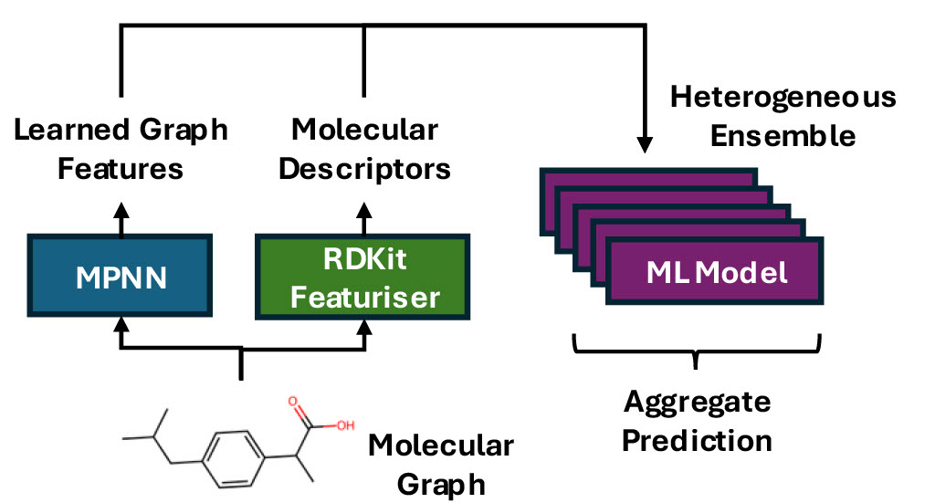
To overcome this challenge, we introduce the MetaModel (Figure 1), an ensemble model constructed by combining the predictions from many different classes of ML algorithms. By weighting the individual sub-model predictions based on their validation set performance, we can ensure that we prioritise the models that perform best on any given problem.
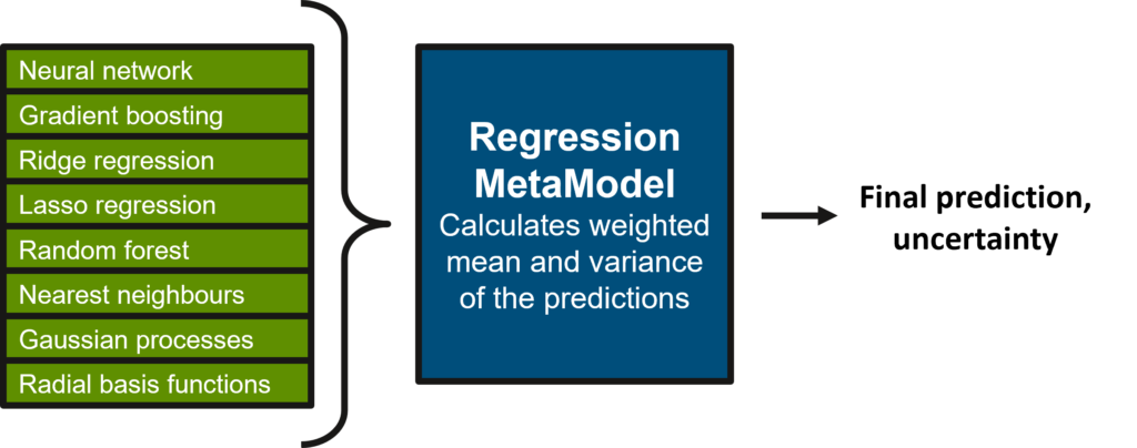
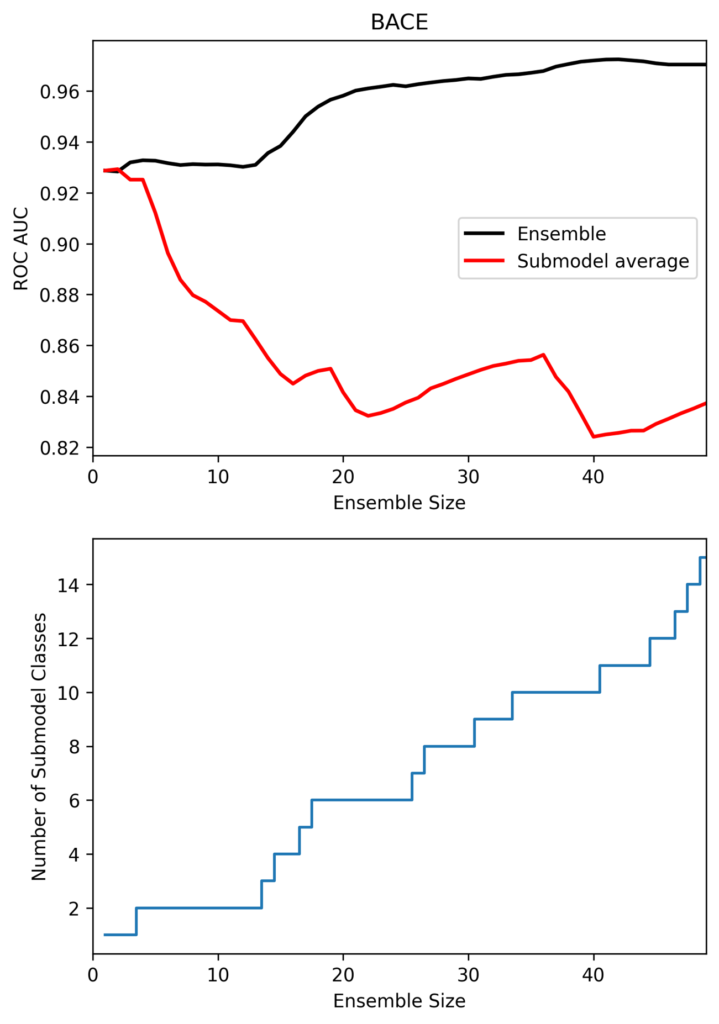
Figure 2 shows the performance of the MetaModel ensemble as a function of the number of sub-models in the ensemble on the MoleculeNet BACE dataset. In this case, smaller ensembles perform worse, even if the average performance of the sub-models in the ensemble is better. The sharp drop in performance below an ensemble size of 20 corresponds to a drop in the number of sub-model classes from 6 to 2, demonstrating the importance of a diverse ensemble of models.
There are additional benefits to this approach:
Now that we have an ensemble that should be able to tackle any modelling problem, how can we set it up for success?
You may already be familiar with the phrase “garbage in, garbage out” as it applies to ML: the final model is only ever as good as the data used to train it. For QSAR modelling, a big part of this is the choice of molecular descriptors. Descriptors are how we convert a compound into a set of numbers, representing different physical or chemical properties of the compound, which can then be used as input to an ML model. Many thousands of different potential descriptors exist, from basic properties like molecular weight to sophisticated 4D descriptors built from molecular dynamics simulations.
Given the abundance of descriptors, one might naively assume that we can shove all of them into our model and let the algorithm figure it out. However, if we try this, we run into the scourge of machine learning: overfitting. Like humans seeing faces in clouds, ML models love to find patterns where none exist. The more numbers we feed them, the more spurious correlations they will find, and the worse they will perform in the real world.
Because of this, we have to pick a relatively small set of descriptors, typically tens to hundreds, to better our chances of identifying real patterns in the data. Unfortunately, just as no single model is optimal across all problems, no one set of descriptors will be optimal. This puts us in a bit of a bind: we can’t use all possible descriptors, and any subset we choose will sometimes be wrong.
Fortunately, we can work around this problem by deriving our own task-specific descriptors. The most popular way to do this is using graph neural networks (GNNs). Like the convolutional networks used for image classification, these models can work directly from the raw data, which in this case are molecular graphs.
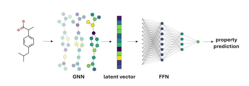
The GNN first derives its own numerical representation of the molecular graph, as a latent vector, before using a feed-forward network (FFN) prediction head to turn that vector into a property prediction. This numerical representation encodes all the relevant information the GNN can find, effectively a learned set of descriptors. These descriptors will be custom-made for the property we’re trying to predict, so we don’t have to worry about pushing irrelevant data into our model.
While this is a big improvement, GNNs do have weaknesses. Firstly, it’s generally not possible to derive all the relevant descriptors from a limited dataset, and GNNs have their own blind spots – they’re very good at understanding local structure, but struggle with global properties. Modern GNNs like ChemProp mitigate this by supplementing their latent vector with general-purpose fixed descriptors, getting the best of both worlds.
The second weakness is inherent to the model architecture – GNNs typically rely on an FFN to turn their descriptors into a property prediction. This is effectively the same as a multi-layer perceptron model, the classic neural network for property prediction, and, as we’ve seen, no single model class will perform optimally across all tasks. Relying purely on FFNs to make predictions limits the potential of GNN-based models, meaning that their powerful molecular representations are not always fully exploited.
In our paper, we show that we can improve on this by extracting the learned descriptors from a trained ChemProp model and using them, and with a set of general-purpose descriptors, as input to the MetaModel ensemble.
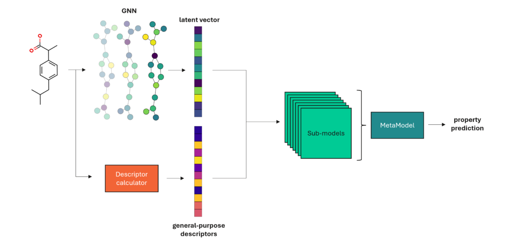
In this way, we get the benefit of task-specific descriptors without the limitations of a pure neural network approach.
We tested our modelling framework on the MoleculeNet datasets, benchmarking the MetaModel performance against ChemProp.
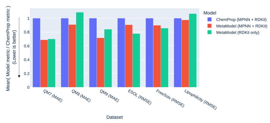
This plot shows the performance of ChemProp and the MetaModel on the six regression datasets (measured using mean absolute error (MAE), or root mean squared error (RMSE), so lower is better). In each case, we test the MetaModel with a set of general-purpose descriptors from RDKit, and either with or without GNN descriptors from a ChemProp message-passing neural network (MPNN). The MetaModel performs better than ChemProp on every dataset, with five of them highly significant, and one marginally (Lipophilicity, p=0.05).
The addition of the GNN/MPNN descriptors is more nuanced, improving the MetaModel performance on the three quantum mechanics datasets but having little or no benefit on the physical chemistry datasets. This is likely because the general-purpose RDKit descriptors are already a good match to the PhysChem datasets, meaning that the learned descriptors are unable to add value.
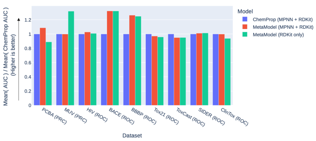
The picture is similar for the nine classification datasets (performance is measured in the AUC of either the ROC curve or the precision recall curve (PRC), so higher is better).
The MetaModel outperforms ChemProp on six datasets (of which three are highly significant), while ChemProp significantly outperforms the MetaModel on the ToxCast and Tox21 datasets. These are large, sparse datasets with many endpoints, which benefit a multi-target model like ChemProp over the single-target MetaModel. In fact, these datasets are much more suited to an imputation model like the one underpinning our Cerella™ deep learning platform!
Aside from these exceptions, where we could not reasonably expect the MetaModel to perform as well, it consistently matches or outperforms ChemProp. This is the sort of behaviour we should anticipate: where ChemProp is already close to optimal, there is no room for improvement, so the best we can do is match it. On the other hand, where ChemProp is underperforming (because the FFN is not the best model for the job), the flexibility of the MetaModel ensemble allows it to find better solutions and make better predictions.
Our work demonstrates the potential for pushing the limits of QSAR modelling using diverse ensemble models, to ensure the best-performing algorithms are prioritised for every task, and by using GNNs as featurisers to extract relevant information from molecular graphs. The paper is published in JCIM, and a pre-print version is available here.
These upgrades will be implemented into our Auto-Modeller™ module, enabling StarDrop users to build and validate their own cutting-edge QSAR models, tailored to their chemistry and data, at the press of a button. Ultimately, these improved models give chemists the tools they need to better understand their molecules and prioritise the right designs for synthesis and testing.
Michael is a Principal AI Scientist at Optibrium, applying advanced AI techniques to accelerate drug discovery and improve decision-making. With a Ph.D. in Astronomy and Astrophysics from the University of Cambridge, he brings a data-driven approach to solving complex scientific challenges. Michael is also a thought leader, contributing to discussions on the impact of AI in pharmaceutical research.

Introduction After training a classification model, we would like to evaluate its performance by using the trained model on an…
Summary In this study, our researchers combined an automatic model generation process for building QSAR models with the Gaussian Processes…

Summary In this study, the researchers look to solve classification quantitative structure−activity relationship (QSAR) modelling problems using Gaussian processes. They…