How do you know the performance of your predictive models? In this blog, Mario will talk you through a simple example using images of cats and dogs. He’ll dive into numbers, charts, and key metrics like Cohen’s Unweighted Kappa and Kappa with Linear Weighting to evaluate the performance of classification models. Read on and discover how to assess your models like a pro!

Introduction

After training a classification model, we would like to evaluate its performance by using the trained model on an external test set. The most straightforward performance indicator would be its accuracy (p), where we would divide the number of correct predictions with the number of total predictions. Accuracy, however, can be misleading when evaluating the usefulness of a classification model. 

Let us consider a task, where we must build a classifier, which detects if an image portrays a cat. After going through the training process, we are confident that our model works, and we would like to test it on an external test set. The dataset for testing the model consists of 100 images – 90 images of cats and 10 images of dogs. Our model predicts that 86 out 100 images contain cats. Unfortunately, in five cases, the model makes a misprediction and labels a dog image as a cat image. However, the number of correct predictions is still 86 – 81 correct predictions when an image contains a cat and 5 correct predictions when an image contains a dog. The p of the model is 0.86 or 86 per cent.  

We can get a visual overview of the model performance by plotting out a confusion matrix, where each row of the matrix represents the species on the images, while each column represents the prediction by the model (Figure 1). For a perfect model the confusion matrix would be a diagonal matrix – the main diagonal of the confusion matrix would contain the numbers 90 and 10, while the off-diagonal elements would be zero. 

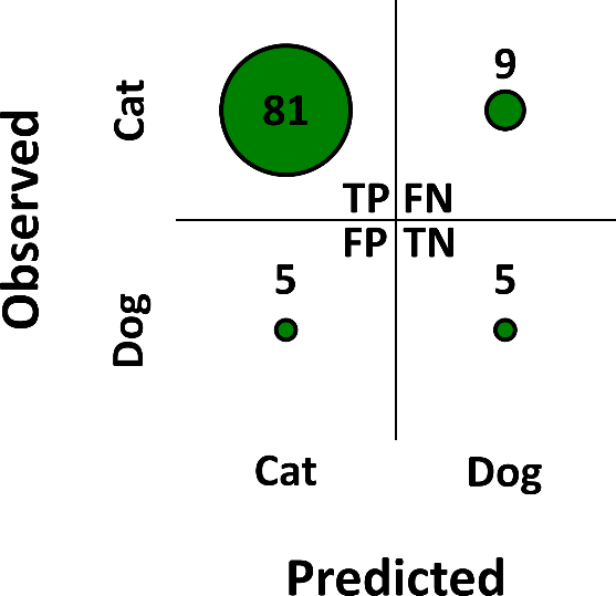
If we would create an arbitrary model, which would classify everything as an image of a cat, we would obtain a p of 0.90 on the same test set. If we would use p as the only performance indicator, then we could say that the arbitrary model is better. However, our intuition should tell us that the arbitrary model is useless, and its performance is only better because of the bias in the external test set. 

In such a case we would benefit from the use of Cohen’s Kappa (κ) as our main performance indicator since it takes into account the bias in the data. Theoretically, the κ value ranges from −1.0 to 1.0 where the higher result refers to a better model. For the aforementioned models, the κ values would be 0.34 and 0.00 for the real classifier and the arbitrary model, respectively. Thus, it is safe to conclude that the trained model is better than the arbitrary model. While the given example was somewhat absurd, it illustrated the pitfall of using p alone for evaluating the usefulness of a classifier using an imbalanced external test set. 

How to Calculate Cohen’s Kappa 

To calculate the κ value, we need to first calculate the chance agreement (p_e) between the actual class values and the predictions. For a binary classification model described above, the p_e is the sum of  

• the probability of the predictions agreeing with the labels in the test set for images of cats (p_e1) and 

• the probability of the predictions agreeing with the labels in the test set for images of dogs (p_e2). 

When calculating the probabilities, we make the assumption that the actual class values and the model predictions are independent. The p_e1 and p_e2 are calculated by multiplying the proportion of the actual class values and the proportion of the predicted class values. For the above model we would receive the following numbers: 

P_{e1} = \frac{(TP + FN) \times (TP + FP)}{Total\,Predictions} = \frac{90 \times 86}{100} = 77.40\%
P_{e2} = \frac{(TN + FP) \times (TN + FN)}{Total\,Predictions} = \frac{10 \times 14}{100} = 1.40\%
P_e = 77.40\% + 1.40\% = 78.80\% = 0.7880

Where TP, TN, FN, and FP stand for true positive (correctly predicted cat images), true negative (correctly predicted dog images), false-negative (mis-predicted cat pictures), and false positive (mis-predicted dog pictures), respectively. 

To calculate the κ value, we need the overall accuracy (p), which was calculated before and the p_e: 

\kappa = \frac{P - P_e}{1 - P_e} = \frac{0.8600 - 0.7880}{1.0000 - 0.7880} = \frac{0.0720}{0.2120} = 0.3396

For the arbitrary model, where the p was 0.90, the p_e2 is 0.00 ((10×0)/ 100); thus, the κ would be 0.00 as well. 

The κ value considers the possibility that the prediction result might agree with the actual class value purely by a chance. The equation represents the ratio between the percentage of predictions, which cannot be explained by a random guess in the trained model and the percentage of predictions, which cannot be explained by a random guess in a perfect model, where the p would be 1.00. The chances of random agreement in a highly biased test sets are quite high, as seen from our example with the presented models; thus, the κ value is better at evaluating the performance than the p value alone. 

How to Interpret the Values of Cohen’s Kappa 

Similarly, to other types of correlation coefficient, the κ value can vary between −1.0 and 1.0. The value of 1.0 represents the perfect agreement between the observed and the predicted values, the value of 0.0 represents the amount of agreement that can be expected from random chance and the value of −1.0, technically, represents the perfect negative correlation between the observed and the predicted values. But how to interpret the κ values and why only values between 0 and 1 are considered to have any useful meaning? 

In the first instance let us explore three data sets, which all have 100 data points – 100 pictures of cats and dogs. The first data set is a balanced data set with 50 pictures of cats and 50 pictures of dogs, the second data set is slightly biased towards cats with 75 pictures of cats and 25 pictures of dogs, and the third data set is heavily biased towards cats with 90 pictures of cats and 10 pictures of dogs. For each data set, we will have a set of hypothetical models, which will mis-predict N number of dog pictures, where N ranges from 0 to the number of dog pictures in the data set. Thus, we can compare the accuracy and the κ value for each model within each data set – Figure 2. 

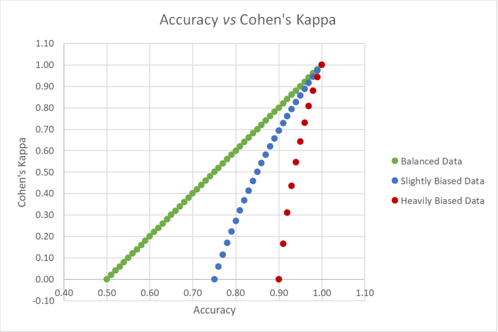
There is a perfect linear correlation between the p and κ values for the models for the balanced data set and when the hypothetical model predicts all 100 pictures to be pictures of cats, the accuracy of the model is 0.5 and the kappa value is 0.0, as expected. However, the biased data sets show a non-linear trend and instances, where p values are high, while κ values approach 0.0 are common. Thus, as said before, the p of a model might be misleading, especially when the test set is heavily biased. 

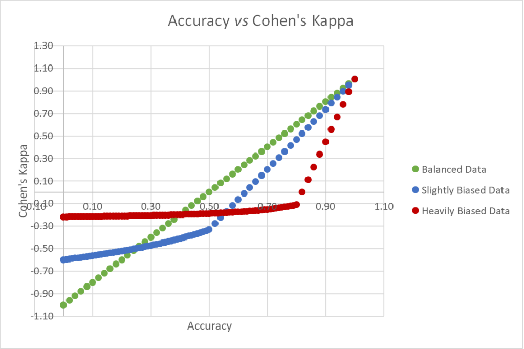
But what would happen if the dog pictures would be mis-classified as cat pictures (as before), while the cat pictures would be mis-classified as dog pictures? We will use the same data sets as before, but this time we will have a set of hypothetical models, which will mis-predict N number of dog pictures and M number of cat pictures, simultaneously, where N and M range from 0 to the number of dog pictures and from 0 to the number of cat pictures, respectively. 

There are few interesting observations, which can be made from the graph – Figure 3. The trendline for the balanced data set did not change at all because it does not matter, which class is mis-predicted as there is an equal number of both cat and dog pictures. Furthermore, the κ values for the balanced data set are the only ones, which reach the theoretical minimum of −1.0. Thus, the fact that the absolute minimum for a κ value depends on the bias in the data set makes it cumbersome to assess if a negative correlation exists in the model or not. Furthermore, it is impossible to compare models with negative correlation, because as can be seen from Figure 3, the perfect negative correlation for a heavily biased data set is approaching −0.22, while for a slightly biased data set it is approaching −0.60. In both cases it is not even close to the theoretical minimum of −1.0. Luckily, the κ values of 0.00 and below are unlikely in practice. The last interesting bit is the fact that for the biased data sets, the κ value is better for models where 5 dog and 5 cat pictures got mis-classified opposed to models where 10 dog pictures got mis-classified. 

As with accuracy values it is complicated to draw a hard line between κ values and state that models with κ values over a certain threshold are good enough. However, scientists have proposed a guide on how to assess your models, which is presented in Table 1. In general, models with a κ value of over 0.60 are considered useful. 

Value of Cohen’s Kappa	Level of Agreement
0.00…0.20	None
0.21…0.39	Minimal
0.40…0.59	Weak
0.60…0.79	Moderate
0.80…0.90	Strong
0.91…1.00	Almost Perfect to Perfect

How to Calculate Cohen’s Kappa for Three or More Categories 

The Cohen’s Kappa can also be calculated for a model with three of more classes. Let us imagine that we have trained a classification model, which classifies images as cats, dogs, or foxes. The external test set has 40 cat images, 40 dog images and 20 fox images and the confusion matrix for the model performance is on Figure 4. The acronyms TC, FCD, FCF, TD, FDC, FDF, TF, FFC, and FFD stand for true cat image (correctly predicted cat images), false cat image (dog mis-predicted as a cat), false cat image (fox mis-predicted as a cat), true dog image, false dog image (cat mis-predicted as a dog), false dog image (fox mis-predicted as a dog), true fox image, false fox image (cat mis-predicted as a fox) and false fox image (dog mis-predicted as a fox), respectively. 

The p_e (chance agreement) for the model with three classes is a sum of p_{e cat}, p_{e dog}, and p_{e fox}. The p_e is found using the following equations: 

P_{e\,cat} = \frac{(TC + FDC + FFC) \times (TC + FCD + FCF)}{Total\,Predictions} = \frac{40 \times 45}{100} = 18.00\%
P_{e\,dog} = \frac{(TD + FCD + FFD) \times (TD + FDC + FDF)}{Total\,Predictions} = \frac{40 \times 35}{100} = 14.00\%
P_{e\,fox} = \frac{(TF + CFC + FDF) \times (TF + FFC + FFD)}{Total\,Predictions} = \frac{20 \times 20}{100} = 4.00\%
P_e = 18.00\% + 14.00\% + 4.00\% = 36.00\% = 0.3600

The p (accuracy) of the model is 81% ((35+29+17)/100)) and the κ is 0.70 ((0.8100−0.3600)/(1.0000−0.3600)), which is a very good result for a model with three classes. In general, it is expected that the κ value for a model with three or more classes is worse than the κ value for a binary classification model. 

The pattern for finding the chance agreements for a model with any number of classes is the following: 

• The p_e is a sum of N probability values of the predictions agreeing with the labels in the test set, where N is the number of classes; 

• The probability values mentioned above are calculated by multiplying the sum of the numbers in the row and the sum of the numbers in the column for each diagonal element¹ of the confusion matrix and dividing each product by the number of total predictions. 

Weighted Cohen’s Kappa 

When we build a classification model where the categories are ordinal, e.g., how spicy a chilly pepper is – mild, medium, and hot, then a situation where a mild pepper is mispredicted to be a medium one is better than it being predicted as hot. In such cases, it would be appropriate to use the weighted κ, where we would take into account the relative concordances – each cell in a row of the matrix is weighted in accordance with how near it is to the cell in that row that includes the absolutely concordant items. 

To understand how the weights work, we should revisit our previous example with cats, dogs, and foxes. We did not explicitly use weights in that example; however, they were present – the weights for the diagonal elements of the confusion matrix were 1 and the weight for every other element in the matrix was 0. In theory, we should have multiplied the accuracy and the chance agreement of the diagonal elements with 1 and the accuracy and the chance agreement of every other element with 0 and then summed the results, respectively. However, since only the diagonal elements yield results other than 0, we skipped the other elements. Such an approach makes sense, because when the observed label is a cat, then a mis-prediction of it to a dog is not better than a mis-prediction of it to a fox and the weights for the elements FCD and FCF on Figure 4 should both be 0. As described in the previous paragraph, the situation changes, when we have ordinal categories. 

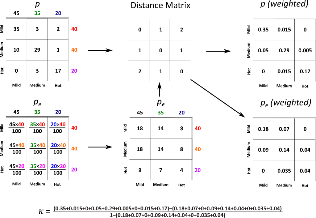
Let us continue with the same confusion matrix, however, let us change the labels cat, dog, and fox to mild, medium, and hot, respectively. With k ordinal categories and equal imputed distances between successive categories, the maximum possible distance between any two categories is k − 1, which in the present example is equal to 2 (3 − 1). This is the general equation for calculating the linear² weights for each element: 

weight = 1 - \frac{|distance|}{maximum\, possible\, distance}

Thus, the weights for the diagonal elements of the aforementioned confusion matrix are 1 (1−(0/2)), the weights for the elements in super- and sub-diagonal would be 0.5 (1−(1/2)), and the weights for the rest of the elements would be 0 (1−(2/2)). To calculate the weighted κ, we need to calculate both the weighted p and the weighted p_e. The results are summed in Figure 5 – as can be seen, the weighted κ (0.74) is slightly higher than the unweighted κ (0.70). Weighted κ values tend to be more difficult to interpret as they are not intuitive to understand compared to unweighted κ values. 

Additional Concepts

We could calculate the standard error and the confidence interval for Cohen’s κ; however, in the context of evaluating a classification model it is not necessary nor common to do it. Thus, the current document does not include the procedure of how to calculate standard errors and confidence intervals. Since the κ value is technically a correlation coefficient it could be squared, which would give us the coefficient of determination. However, the interpretation of κ² is not straightforward and such an operation has been described in only one publication. 

Useful Publications and Links 

J. Cohen, “A Coefficient of Agreement for Nominal Scales”, Educational and Psychological Measurement, 1960, 20, 37-46. 

J. Cohen, “Weighted Kappa: Nominal Scale Agreement with Provision for Scaled Disagreement or Partial Credit”, Psychological Bulletin, 1968, 70, 213-220. 

M. L. McHugh, “Interrater reliability: the kappa statistic”, Biochemia Medica, 2012, 22(3), 276-282. 

http://www.vassarstats.net/kappa.html

https://www.real-statistics.com/reliability/interrater-reliability/cohens-kappa/

https://www.real-statistics.com/reliability/interrater-reliability/weighted-cohens-kappa/

https://thenewstack.io/cohens-kappa-what-it-is-when-to-use-it-and-how-to-avoid-its-pitfalls

Want to learn more?

In this recorded webinar, Dr Tamsin Mansley and Dr Mario Oeren explored the art of predictive modelling for drug discovery. Watch and learn key ADME properties to predict with in silico models, the four pillars of quality model building and how to build and validate robust QSAR models tailored to your data, with a live demo of StarDrop’s Auto-Modeller software.

About the author

Mario Öeren, PhD

Mario is a Principal Scientist at Optibrium, where he applies expertise in quantum chemistry, conformational analysis, and molecular modeling to support drug discovery research. With a PhD in Natural Sciences from Tallinn University of Technology, his academic work focused on computational studies of macrocyclic molecules. Mario has authored numerous publications and has extensive experience in chemical education and advanced spectroscopy.

Linkedin

More predictive modelling resources

On-demand

Multi-parameter optimisation in practice

This webinar describes example applications of multi-parameter optimisation to find high-quality lead compounds.

Multi-parameter optimisation

8 September 2020

Guided multi-parameter optimisation of 2D and 3D SAR

This SeeSAR and ADME QSAR worked example uses a combination of 2D and 3D methods to understand and optimise a virtual library of Heat Shock Protein 90 (HSP90) inhibitors.

Predictive modelling

18 May 2022

Gaussian processes for classification: QSAR modeling of ADMET and target activity

Summary In this study, the researchers look to solve classification quantitative structure−activity relationship (QSAR) modelling problems using Gaussian processes. They…

Exploring structure-activity relationships

4 May 2010