Automatic QSAR modeling of ADME properties: blood-brain barrier penetration and aqueous solubility
Summary In this study, our researchers combined an automatic model generation process for building QSAR models with the Gaussian Processes…

My hope is that these posts will be of interest to people who want to understand more of the nuts and bolts of how ML modelling works. If this sounds like torture to you, I can recommend several higher-level blog posts from my colleagues. If you’re just interested in being confident that Optibrium’s models work, for instance, read Mario’s blog. Or if you want to know how to gain the most value from your models, try Daniel’s blog.
The first step in building a QSAR model is to decide what you want to predict. The next is to find or make some relevant data, and clean it. I will skip over most of this, because it’s boring, but this can easily be 90% of the process. For this demo, I’m going to use the Caco-2 dataset from Wang et al. 2016 but the pre-cleaned version from Therapeutic Data Commons.
In Python, we can read our clean and shiny data using the pandas library:

We could, in principle, build a model to predict the QSAR property from the SMILES string directly using some kind of chemical language model. However, this is generally going to be quite inefficient in training time and computing cost, and is unlikely to be competitive (we might still do this in a later blog post, just because it’s fun). A better (cheaper/faster/more accurate) approach is to use a set of molecular descriptors. These are numerical values describing simple properties of the molecule, which can be derived from the SMILES string, as input to our machine learning model.
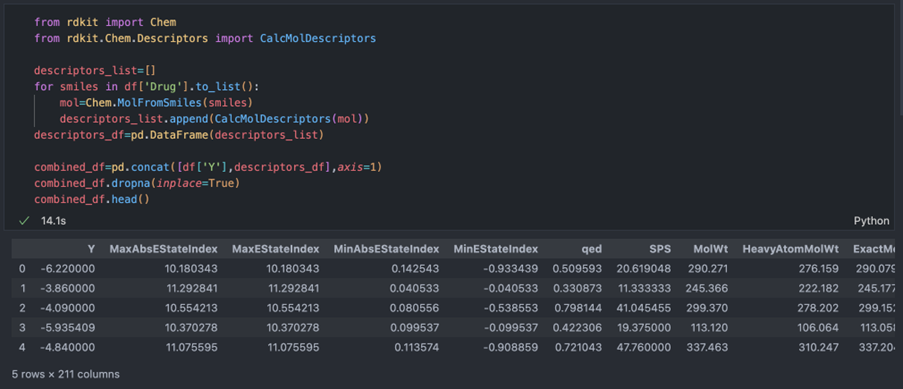
Our in-house models use our own set of custom descriptors, but for this demo, I’ll use the rdkit library to derive descriptors for each compound in the dataset:
I’ve concatenated the descriptor dataframe with the target value from our data, so now for each compound, we have 210 descriptors and 1 Y value. We have one final step to go through before we can actually train our model: splitting the data into training and test sets.

This is a very important step, because otherwise, we cannot accurately assess how our model is performing. If we just look at how accurate the model is on the data we used to train it, it may appear to be performing very well. However, it might in fact just have memorised the training data, and have no real predictive value. By having a test set of compounds that the model hasn’t seen during training, we can get a more accurate picture of how it’s likely to do in the real world. For this, we can use scikit-learn, a great general-purpose ML library:

Now we’re finally ready to train our model! I’m going to use a random forest, because they’re simple, effective, and fast. Again, we can use scikit-learn for this, and I’m going to use the default model parameters (I’ll address selecting and optimising hyperparameters in a future blog post).

We have our trained model, but how good is it? To evaluate this, we can use the test set that we set aside earlier, comparing the model’s predictions for the test set with the true values that it hasn’t seen:

We get a test-set R2 (see Mario’s blog) of 0.7. That’s not bad, considering we put no effort whatsoever into optimising either our descriptors or model. The test-set R2 reported by Wang et al. is 0.81, so we still have room for improvement, but it’s pretty good for a first go.
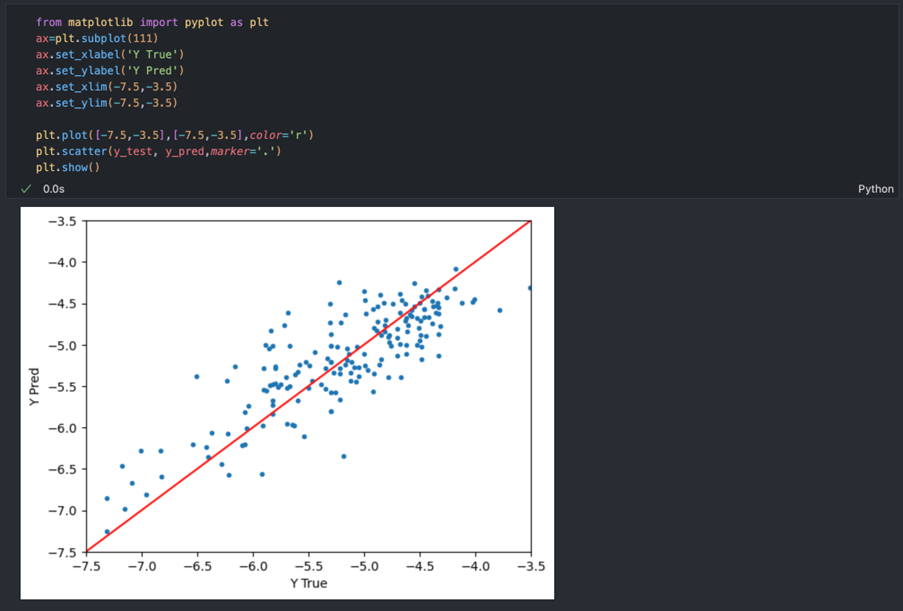
To get a closer look at the model performance, and to spot things that might cause us problems, we can plot the predicted Caco-2 value against the true value for the test set. For this, we can use matplotlib. It’s always worth actually looking at the data where possible, rather than relying solely on metrics. Otherwise, you can miss important things. In this case, the results look encouraging:

There’s clearly a nice correlation between the true and predicted y values. Furthermore, nothing stands out as looking weird, so that’s good. Whilst there’s room for improvement, as indicated by quite a bit of scatter around the 1:1 line, overall we can call this a success.
Our ADME QSAR models and Auto-Modeller software are far more sophisticated than the simple demo we’ve worked through here. However, they rely on the same underlying processes. The StarDrop ADME QSAR module provides pre-built, high-quality predictive QSAR models of a broad range of key ADME and physicochemical properties.
The Auto-Modeller module enables you to build and validate robust QSAR models tailored to your chemistry and data, in an easy and intuitive way. It is highly automated, guiding you through the data set splitting, model building, and validation steps using multiple machine learning methods. This means that, even if you’re not an expert, you can build and validate robust models of your data, without needing to dive into Python yourself. If you’re interested, you can see an example of Auto-Modeller in action here.
Next time, I’ll look at how to train your first neural network.
We would love to show you how StarDrop can help your drug discovery projects. Complete the form and a member of the team will get in touch to arrange a personalised demo for you.
Michael is a Principal AI Scientist at Optibrium, applying advanced AI techniques to accelerate drug discovery and improve decision-making. With a Ph.D. in Astronomy and Astrophysics from the University of Cambridge, he brings a data-driven approach to solving complex scientific challenges. Michael is also a thought leader, contributing to discussions on the impact of AI in pharmaceutical research.

Summary In this study, our researchers combined an automatic model generation process for building QSAR models with the Gaussian Processes…

In this webinar, we examine the effective use of QSAR modelling in drug discovery and discuss a variety of pain points for medicinal chemists in knowing when a model can be trusted and how to avoid common pitfalls.

During this example we will consider three compounds from a lead series which we would like to try to evolve into a candidate. The compound has a good profile of ADME properties but insufficient inhibition of the target, the Serotonin transporter. In this example we will use StarDrop’s Nova module to generate new ideas for compounds to improve the potency while maintaining the balance of other properties.
