Pushing the limits of QSAR modelling
Probably the most common use of machine learning (ML) in drug discovery is QSAR modelling, where we predict the properties…
Good statistics don’t guarantee good applicability. Performance metrics will tell you how well a QSAR model predicts known data, but they don’t tell you whether it will add practical value when applied to your project.
In some cases, even models that appear excellent on paper can fall short, leaving you with almost as much experimental work as you would have had without the model in the first place.
In this blog, we’ll explore why you should look beyond the statistics and how to assess whether a model will genuinely add value to your research.
Let’s consider a classification model for identifying active compounds.
Imagine you’ve evaluated it using the area under the ROC curve (AUC-ROC), which measures how well a model distinguishes between classes, with values ranging from 0 to 1.0, with 0.5 being the equivalent to random. Your model achieves a result of 0.85, which is a strong outcome. The sensitivity (the proportion of true actives correctly identified) is 70%, and the false positive rate (the proportion of inactive compounds incorrectly flagged as active) is 20%. These statistics suggest you have a reliable model.
Now, imagine you’re applying this model in early-stage virtual screening to a compound library of 500,000 to 1 million compounds, or even more. You decide to screen 10,000 candidates in silico. Here’s where you need to consider the base rate.
In early-stage virtual screening, the proportion of active compounds is typically very small. Let’s say 0.5% of your library contains actives (in reality, it could be as low as 0.1%). With 10,000 compounds screened, you’d expect 50 active molecules.
Your model, with 70% sensitivity, identifies 35 of these 50 actives. Excellent. But with a 20% false positive rate, it also flags 1,990 of the 9,950 inactive compounds as active. That means you’d need to experimentally test approximately 2,025 compounds to find those 35 true actives.
If your lab capacity is 1,000 compounds, you’d only identify around 17 true actives from that batch. Even with a statistically robust model, you’re still facing substantial experimental work to extract meaningful results.
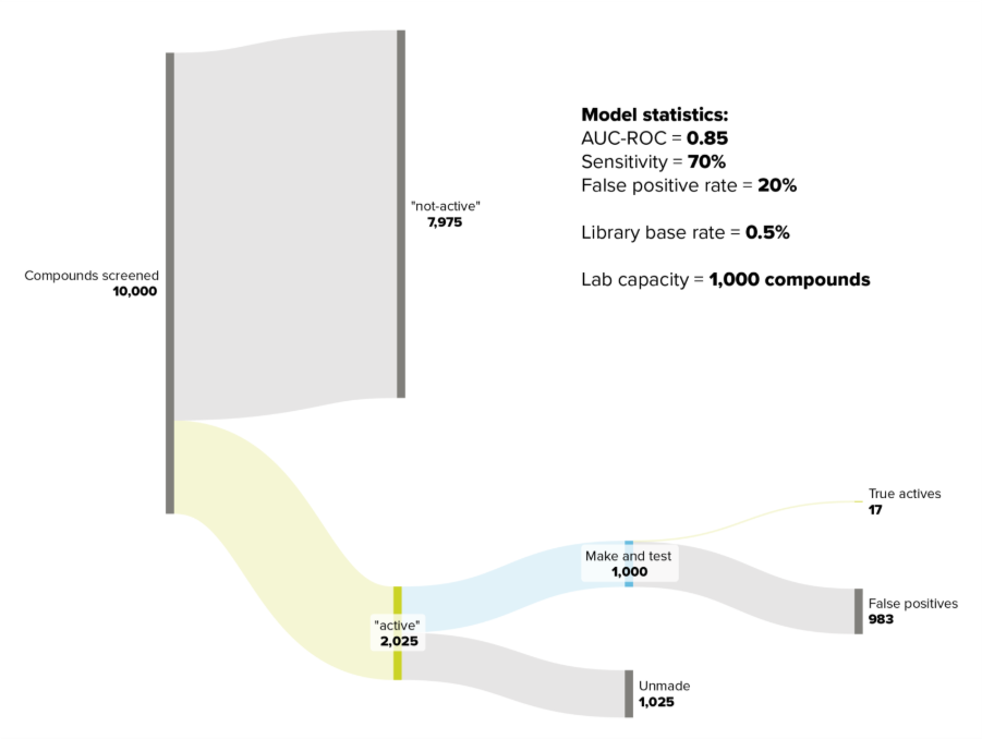
The issue isn’t necessarily that your model is poor; it’s the base rate. When you’re working with highly imbalanced datasets where active compounds are rare, even good models won’t necessarily be able to reduce the experimental burden significantly. If your dataset were balanced (50% active, 50% inactive), this wouldn’t be a problem. But that’s rarely the reality in early drug discovery.
Statistical metrics can sometimes mask limitations in how a model performs across different classes.
A good example of this is a real classification model we previously developed at Optibrium, which categorised compounds into three classes based on their likelihood of being an inhibitor: low, moderate, or high.
We trained the model and evaluated it using a weighted Cohen’s Kappa, which came out at 0.66. That’s generally considered reasonable performance.
However, when we examined the confusion matrix more closely, we discovered a critical issue. The model was excellent at distinguishing between “low” and “moderate” classes. But the compounds in the high category were often classified as “low” or “moderate”.
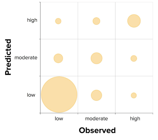
In other words, we had a great model for differentiating between the “low” and “moderate” labels, but no reliable way of identifying whether a compound was an inhibitor with a high likelihood, which was precisely what would be needed for any discovery project. This is because the training dataset itself was somewhat biased; most examples were either “low” or “moderate”, with relatively few examples with the label “high”.
Looking solely at the Kappa value would have led us to believe we had a useful model, but it simply didn’t work for its intended purpose.
As well as gauging overall performance, it’s important to understand how your model performs within each class to determine if it will actually address the question you’re trying to answer.
Even if your model performs well statistically and handles class imbalances appropriately, there’s another potential pitfall: chemical space coverage.
QSAR models are inherently local. They learn patterns from the training data and generalise within the chemical space represented by that data. If you apply your model to compounds that are structurally dissimilar to anything in your training set, predictions become unreliable.
This is particularly problematic when using models trained by colleagues or from external sources, where you may have limited visibility into the training set composition. Without knowing the boundaries of the model’s domain of applicability, you can’t confidently assess whether your compounds fall within it.
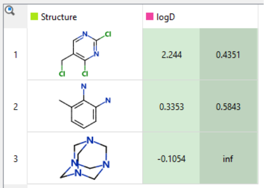
At Optibrium, we address this by providing confidence estimates with all predictions. In StarDrop, every prediction comes with a value that reflects its uncertainty. When this range becomes very large, or even reaches infinity, it signals that you’re likely applying the model to a compound unlike anything in the training set. That’s a warning sign that the prediction may not be trustworthy.
So how do you determine if a model will actually be useful before investing significant time and resources?
Know your data. Before building a model, thoroughly explore your dataset. Look for biases, understand the distribution of your target variable, and examine its chemical diversity. For regression models, consider whether log-transforming your values would be appropriate. Understanding your data upfront helps you anticipate potential issues.
Consider your use case. Once the model is built, think carefully about how it will be applied. What decisions will it inform? What’s the baseline rate in your screening library? Are there class imbalances that could undermine its practical utility? Good statistics may not be sufficient if they don’t translate to meaningful reductions in experimental work.
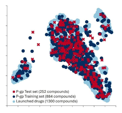
Assess chemical space coverage. Compare your training set to broader reference datasets. At Optibrium, we often use a database of 1,300 marketed drugs to assess coverage. If your training set populates a large portion of that space, you likely have a global model suitable for most drug-like compounds. If it occupies only a small region, it’s a local model, valuable for specific compound classes but not universally applicable. Make sure your model documentation reflects this.
Always check prediction confidence. Every prediction should be accompanied by an uncertainty estimate. If the uncertainty is large, treat that prediction with appropriate scepticism. Uncertainty estimates help you make informed decisions about which predictions you can trust and which require experimental validation. You can learn more about how you can leverage uncertainties to identify even better compounds in our on-demand webinar.
QSAR models are powerful tools, but they’re not magic. A model with good statistics can still fail to deliver practical value if the base rate is unfavourable, if class imbalances aren’t properly addressed, or if it’s applied outside its chemical space.
The key is to look beyond the numbers. Understand your data, assess how the model will be used, and always consider prediction confidence. By taking these steps, you’ll be better positioned to determine whether a model will genuinely add value to your project, or whether it might leave you with more work than you anticipated.
Principal Scientist
Mario is a Principal Scientist at Optibrium with deep expertise in computational chemistry. He holds a PhD in Natural Sciences from Tallinn University of Technology, where he focused on advanced modelling approaches.
Since joining Optibrium in 2017, Mario has driven key research and development in metabolism prediction, creating next-generation models that bring together quantum mechanics and machine learning to support more confident discovery decisions.

Probably the most common use of machine learning (ML) in drug discovery is QSAR modelling, where we predict the properties…
Summary In this study, the researchers look to solve classification quantitative structure−activity relationship (QSAR) modelling problems using Gaussian processes. They…

Introduction After training a classification model, we would like to evaluate its performance by using the trained model on an…