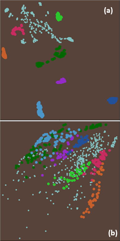
The x- and y-axis are not labelled because the visual clustering method being used is a nonlinear reduction algorithm attempting to take high-dimensional data (multidimensional data in more than three dimensions) and then display the relationships in only two or three dimensions.
Visual clustering
Visual clustering uses an approach known as t-SNE (t-distributed Stochastic Neighbour Embedding). t-SNE is a nonlinear dimensionality reduction algorithm ideally suited to visualising high-dimensional data in two or three dimensions. The algorithm starts by converting the high- and low-dimensional similarities between n compounds into a set of joint probabilities. In high-dimensional space, conditional probabilities are calculated based on Gaussians centred at each high-dimensional point x_i:

which are then symmetrised to form joint probabilities

The low-dimensional probabilities are computed based on Student’s t-distribution:

where the yis are the low-dimensional points.
The Kullback-Leibler divergence between these high- and low-dimensional joint probability distributions P and Q is given by

and is then minimised over the low-dimensional points to obtain a clustering of low-dimensional points in which similar compounds are placed close together and dissimilar compounds are far apart (van der Maaten & Hinton, 2008)
As can be seen in Figure 3‑3, t-SNE tends to produce superior visualisations to PCA. However, it is much more computationally expensive. As a nonparametric technique t-SNE does not provide us with a mapping that we can use to project new data sets into an existing chemical space; in our implementation, we work around this problem by “learning” a parameterised projection post hoc from the high-dimensional compounds and their low-dimensional counterparts. This approach is also used to enable t-SNE to automatically scale to much larger data sets by first using a random sample of the original set of compounds to compute a parameterised projection, and then applying this projection to the remaining compounds.

Additional info:
Some basic rules to help interpret the plots are:
- A chemical space plot allows you to visualize trends across a data set.
- Each point represents one compound.
- The closer two points are, the greater their similarity are in Structure and Properties.
- A single data set defines a space, but other data sets can be plotted in that space simultaneously to explore their overlap.